Lissom
The LISSOM model focuses on V1 and the structures to which it connects. This note explains the key concepts of the LISSOM networks: its architecture, activation and learning rule.
LISSOM principles
LISSOM is a laterally connected map model of the Primary Visual Cortex . The model is based on self-organizing maps, but its connectivity, activation, and learning mechanisms are designed to capture the essential biological processes in more detail.
LISSOM is based on five principles:
- The central layout of the LISSOM model is a two-dimensional array of computational units, corresponding to vertical columns in the cortex. Such columns act as functional units in the cortex, responding to similar inputs, and therefore form an appropriate level of granularity for a functional model.
- Each unit receives input from a local anatomical receptive field in the retina, mediated by the ON-center and OFF-center channels of the LGN. Such connectivity corresponds to the neural anatomy; it also allows modeling a large area of the visual cortex and processing large realistic visual inputs, which in turn allows studying higher visual function such as visual illusions, grouping, and face detection.
- The cortical units are connected with excitatory and inhibitory lateral connections that adapt as an integral part of the self-organizing process.
- The units respond by computing a weighted sum of their input, limited by a logistic (sigmoid) nonlinearity. This is a standard model of computation in the neuronal units that matches their biological characteristics well.
- The learning is based on Hebbian adaptation with divisive normalization. Hebbian learning is well supported by neurobiological data and biological experiments have also suggested how normalization could occur in animals.
In other words, LISSOM takes the central idea of self-organizing maps (1), and implements it at a level of known visual cortex structures (2 and 3) and processes (4 and 5). Although each of these principles has been tested in other models, their combination is novel and allows LISSOM to account for a wide range of phenomena in the development, plasticity, and function of the primary visual cortex.
The LISSOM model
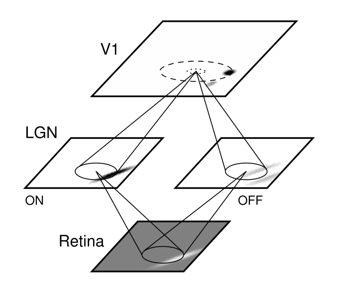
Basic LISSOM model of the primary visual cortex. The core of the LISSOM model consists of a two-dimensional array of computational units representing columns in V1. These units receive input from the retinal receptors through the ON/OFF channels of the LGN, and from other columns in V1 through lateral connections. The solid circles and lines delineate the receptive fields of two sample units in the LGN and one in V1, and the dashed circle in V1 outlines the lateral connections of the V1 unit. The LGN and V1 activation in response to a sample input on the retina is displayed in gray-scale coding from white to black (low to high).
The V1 network in LISSOM is a sheet of N x N interconnected computational units, or “neurons”. Because the focus is on the two-dimensional organization of the cortex, each neuron in V1 corresponds to a vertical column of cells through the six layers of the biological cortex. This columnar organization helps make the problem of simulating such a large number of neurons tractable, and is viable because the cells in a column generally fire in response to the same inputs. The activity of each neuron is represented by a continuous number within [0..1]. Therefore, it is important to keep in mind that LISSOM neurons are not strictly identifiable with single cells in the biological cortex; instead, LISSOM models biological mechanisms at an aggregate level.
Each cortical neuron receives external input from two types of neurons in the LGN: ON-center and OFF-center. The LGN neurons in turn receive input from a small area of the retina, represented as an R x R array of photoreceptor cells. The afferent input connections from the retina to LGN and LGN to V1 are all excitatory. In addition to the afferent connections, each cortical neuron has reciprocal excitatory and inhibitory lateral connections with other neurons. Lateral excitatory connections have a short range, connecting only close neighbors in the map. Lateral inhibitory connections run for long distances, but may be patchy, connecting only selected neurons.
The ON and OFF neurons in the LGN represent the entire pathway from photoreceptor output to the V1 input, including the ON/OFF processing in the retinal ganglion cells and the LGN. Although the ON and OFF neurons are not always physically separated in the biological pathways, for conceptual clarity they are divided into separate channels in LISSOM. Each of these channels is further organized into an L x L array corresponding to the retinotopic organization of the LGN. For simplicity and computational efficiency, only single ON and OFF channels are used in LISSOM, but multiple channels could be included to represent different spatial frequencies. Also, the photoreceptors are uniformly distributed over the retina; since the inputs are relatively small in the most common LISSOM experiments, the fovea/periphery distinction is not crucial for the basic model.
Each neuron develops an initial response as a weighted sum (scalar product) of the activation in its afferent input connections. The lateral interactions between cortical neurons then focus the initial activation pattern into a localized response on the map. After the pattern has stabilized, the connection weights of cortical neurons are modified. As the self-organization progresses, these neurons grow more nonlinear and weak connections die off. The result is a self-organized structure in a dynamic equilibrium with the input.
The following subsections describe the specific components of the LISSOM model in more detail. They focus on the basic version of the model trained with unoriented Gaussian inputs, to highlight the basic principles as clearly as possible.
Connections to the LGN
LISSOM focuses on learning at the cortical level, so all connections to neurons in the ON and OFF channels are set to fixed strengths.
The strengths were chosen to approximate the receptive fields that have been measured in adult LGN cells, using a standard difference-of-Gaussians model. First, the center of each LGN receptive field is mapped to the location in the retina corresponding to the location of the LGN unit. This mapping ensures that the LGN will have the same two-dimensional topographic organization as the retina. Using that location as the center, the weights are then calculated from the difference of two normalized Gaussians. More precisely, the weight \(L_{xy,ab}\) from receptor (x, y) in the receptive field of an ON-center cell (a, b) with center \((x_c,y_c)\) is given by the following equation, where \(\sigma_c\) determines the width of the central Gaussian and \(\sigma_s\) the width of the surround Gaussian:
The weights for an OFF-center cell are the negative of the ON-center weights, i.e. they are calculated as the surround minus the center. shows examples of such ON and OFF receptive fields. Note that even though the OFF cells have the same weights as ON cells (differing only by the sign), their activities are not redundant. Since the firing rates in biological systems cannot be negative, each cell is thresholded to have only positive activations. As a result, the ON and OFF cells will never be active at the same cortical location. They therefore provide complementary information, both in the model and in the visual system. Separating the ON and OFF channels in this way makes it convenient to compare the model with experimental results.
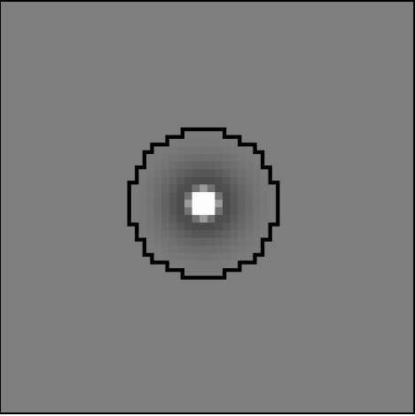
ON neuron
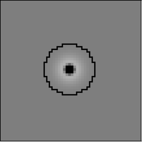
OFF neuron
Connections in the Cortex
In contrast to the fixed connection weights in the LGN, all connections in cortical regions in LISSOM are modifiable by neural activity. They are initialized according to the gross anatomy of the visual cortex, with weight values that provide a neutral starting point for self-organization.
Each neuron’s afferent receptive field center is located randomly within a small radius of its optimal position, i.e. the point corresponding to the neuron’s location in the cortical sheet. The neuron is connected to all ON and OFF neurons within radius rA from the center. For proper self-organization to occur, the radius rA must be large compared with the scatter of the centers, and the RFs of neighboring neurons must overlap significantly, as they do in the cortex.
Lateral excitatory connections are short range, connecting each neuron to itself and to its neighbors within a close radius. The extent of lateral excitation should be comparable to the activity correlations in the input. Lateral inhibitory connections extend in a larger radius, and also include connections from the neuron itself and from its neighbors. The range of lateral inhibition may vary as long as it is greater than the excitatory radius. This overall center–surround pattern is crucial for self-organization, and approximates the lateral interactions that take place at high contrasts in the cortex.
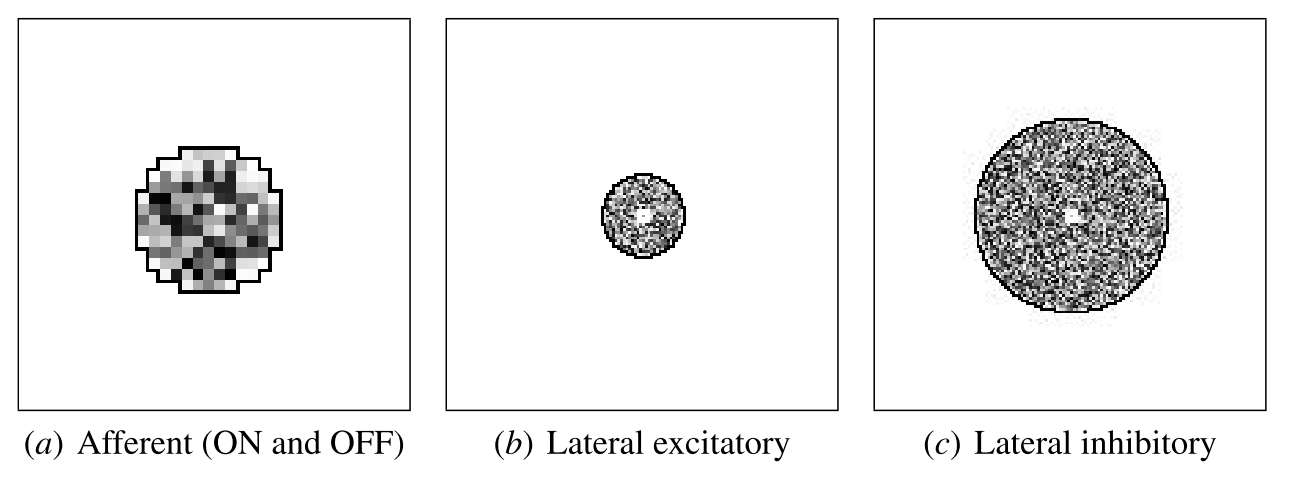
Initial V1 afferent and lateral weights. The initial incoming weights of a sample neuron at the center of V1 are plotted in gray-scale coding from white to black (low to high).
Response Generation
Before each input presentation, the activities of all units in the LISSOM network are initialized to zero. The system then receives input through activation of the retinal units. The activity propagates through the ON and OFF channels of the LGN to the cortical network, where the neurons settle the initial activation through the lateral connections, as will be described in detail below.
Retinal Activation
An input pattern is presented to the LISSOM model by activating the photoreceptor units in the retina according to the gray-scale values in the pattern. shows a basic input pattern consisting of multiple unoriented Gaussians. To generate such input patterns, the activity for photoreceptor cell (x, y) is calculated according to:
where \((x_{c,k},y_{c,k})\) specifies the center of Gaussian \(k\) and \(\sigma_u\) its width. At each iteration, \(x_{c,k}\) and \(y{c,k}\) are chosen randomly within the retinal area; \(\sigma_u\) is usually constant.
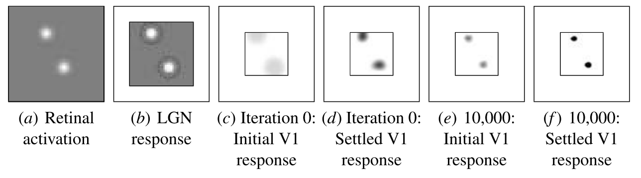
Example input and response. At each self-organization iteration in LISSOM, the photoreceptors in the retina are activated with two unoriented Gaussians.
LGN Activation
The cells in the ON and OFF channels of the LGN compute their responses as a squashed weighted sum of activity in their receptive fields (). More precisely, the response \(\xi_{ab}\) of ON or OFF-center cell \((a, b)\) is calculated as
where \(X_{xy}\) is the activation of cell \((x, y)\) in the receptive field of \((a, b)\), \(L_{xy,ab}\) is the afferent weight from \((x, y)\) to \((a, b)\), and \(\gamma_L\) is a constant scaling factor. The squashing function \(\sigma(\cdot)\) () is a piecewise linear approximation of the sigmoid activation function:
As in other models, this approximation is used because it implements the essential thresholding and saturation behavior, and can be computed more quickly than a smooth logistic function.
Changing \(\gamma_L\) in by a factor \(m\) is equivalent to dividing \(\Theta_l\) and \(\Theta_u\) by \(m\). Even so, \(\gamma_L\) is treated as a separate parameter to make it simpler to use the same values of \(\Theta_l\) and \(\Theta_u\) for different networks. The specific value of \(\gamma_L\) is set manually so that the LGN outputs approach 1.0 in the highest-contrast regions of typical input patterns. This allows each subsequent level to use similar parameter values in general, other than \(\gamma_L\).
Because of its DoG-shaped receptive field, an LGN neuron will respond whenever the input pattern is a better match to the central portion of the RF than to the surrounding portion. The positive and negative portions of the RF thus have a push– pull effect. That is, even if an input pattern activates the ON portion of the LGN RF, the neuron will not fire unless the OFF portion is not activated. This balance ensures that the neurons will remain selective for edges over a wide range of brightness levels. This push–pull effect is crucial when natural images are used as input to the model. Overall, the LGN neurons respond to image contrast, subject to the minimum and maximum activity values enforced by the activation function.
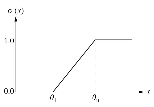
Neuron activation function :math:`sigma(s)`. The neuron requires an input as large as the threshold \(\sigma_l\) before responding, and saturates at the ceiling \(\sigma_u\). The output activation values are limited to [0..1]. This activation function is an efficient approximation of the logistic (sigmoid) function.
Cortical Activation
The cortical activation mechanism is similar to that of the LGN, but extended to support self-organization and to include lateral interactions. The total activation is computed by combining the afferent and lateral contributions. First, the afferent stimulation \(s_{ij}\) of V1 neuron \((i, j)\) is calculated as a weighted sum of activations in its receptive fields on the LGN:
where \(\xi_{ab}\) is the activation of neuron (a, b) in the receptive field of neuron (i, j) in the ON or OFF channels, \(A_{ab,ij}\) is the corresponding afferent weight, and \(\gamma_A\) is a constant scaling factor. The afferent stimulation is squashed using the sigmoid activation function, forming the neuron’s initial response as
After the initial response, lateral interaction sharpens and strengthens the cortical activity over a very short time scale. At each of these subsequent discrete time steps, the neuron combines the afferent stimulation \(s\) with lateral excitation and inhibition:
where \(\eta_{kl}(t - 1)\) is the activity of another cortical neuron (k, l) during the previous time step, \(E_{kl,ij}\) is the excitatory lateral connection weight on the connection from that neuron to neuron (i, j), and \(I_{kl,ij}\) is the inhibitory connection weight. All connection weights have positive values. The scaling factors \(\gamma_E\) and \(\gamma_I\) represent the relative strengths of excitatory and inhibitory lateral interactions, which determine how easily the neuron reaches full activation.
The cortical activity pattern starts out diffuse and spread over a substantial part of the map (). Within a few iterations of , it converges into a small number of stable focused patches of activity, or activity bubbles (). Such settling results in a sparse final activation, which allows representing visual information efficiently. It also ensures that nearby neurons have similar patterns of activity and therefore encode similar information, as seen in the cortex.
Learning
Self-organization of the connection weights takes place in successive input iterations. Each iteration consists of presenting an input image, computing the corresponding settled activation patterns in each neural sheet, and modifying the weights.Weak lateral connections are periodically removed, modeling connection death in biological systems.
Weight Adaptation
After the activity has settled, the connection weights of each cortical neuron are modified. Both the afferent and lateral weights adapt according to the same biologically motivated mechanism: the Hebb rule with divisive postsynaptic normalization:
where \(w_{pq,ij}\) is the current afferent or lateral connection weight (either \(A\), \(E\) or \(I\)) from (p, q) to (i, j), \(w'_{pq,ij}\) is the new weight to be used until the end of the next settling process, \(\alpha\) is the learning rate for each type of connection (\(\alpha_A\) for afferent weights, \(\alpha_E\) for excitatory, and \(\alpha_I\) for inhibitory), \(X_{pq}\) is the presynaptic activity after settling (\(\xi\) for afferent, \(\eta\) for lateral), and \(\eta_{ij}\) stands for the activity of neuron (i, j) after settling. Afferent inputs (i.e. both ON and OFF channels together), lateral excitatory inputs, and lateral inhibitory inputs are normalized separately.
In line with the Hebbian principle, when the presynaptic and postsynaptic neurons are frequently simultaneously active, their connection becomes stronger. As a result, the neurons learn correlations in the input patterns. Normalization prevents the weight values from increasing without bounds; this process corresponds to redistributing the weights so that the sum of each weight type for each neuron remains constant. Such normalization can be seen as an abstraction of neuronal regulatory processes.
Connection Death
Modeling connection death in the cortex, lateral connections in the LISSOM model survive only if they represent significant correlations among neuronal activity. Once the map begins to organize, most of the long-range lateral connections link neurons that are no longer simultaneously active. Their weights become small, and they can be pruned without disrupting self-organization.
The parameter \(t_d\) determines the onset of connection death. At \(t_d\), lateral connections with strengths below a threshold wd are eliminated. From \(t_d\) on, more weak connections are eliminated at intervals \(\Delta t_d\) during the self-organizing process. Eventually, the process reaches an equilibrium where the mapping is stable and all lateral weights stay above \(w_d\). The precise rate of connection death is not crucial to selforganization, and in practice it is often sufficient to prune only once, at \(t_d\).
Most long-range connections are eliminated this way, resulting in patchy lateral connectivity similar to that observed in the visual cortex. Since the total synaptic weight is kept constant, inhibition concentrates on the most highly correlated neurons, resulting in effective suppression of redundant activation. The short-range excitatory connections link neurons that are often part of the same bubble. They have relatively large weights and are rarely pruned.
Parameter Adaptation
The above processes of response generation, weight adaptation, and connection death are sufficient to form ordered afferent and lateral input connections like those in the cortex. However, the process can be further enhanced with gradual adaptation of lateral excitation, sigmoid, and learning parameters, resulting in more refined final maps.
As the lateral connections adapt, the activity bubbles in the cortex will become more focused, resulting in fine-tuning the map. As in other self-organizing models (such as SOM), this process can be accelerated by gradually decreasing the excitatory radius until it covers only the nearest neighbors. Such a decrease helps the network develop more detailed organization faster.
Gradually increasing the sigmoid parameters \(\Theta_l\) and \(\Theta_u\) produces a similar effect. The cortical neurons become harder to activate, further refining the response. Also, the learning rates \(\alpha_A\), \(\alpha_E\) and \(\alpha_I\) can be gradually reduced.
Such parameter adaptation models the biological processes of maturation that take place independently from input-driven self-organization, leading to loss of plasticity in later life.
Supervised Learning
In addition to providing a precise understanding of the mechanisms underlying visual processing in the brain, LISSOM can serve as a foundation for artificial vision systems. Such systems have the advantage that they are likely to process visual information the same way humans do, which makes them appropriate for many practical applications.
First, LISSOM networks can be used to form efficient internal representations for pattern recognition applications. A method must be developed for automatically identifying active areas in the maps and assigning labels to neural populations that respond to particular stimulus features. One particularly elegant approach is to train another neural network to do the interpretation. By adding backprojections from the interpretation network back to the map, a supervised process could be implemented. The backprojections learn which units on the map are statistically most likely to represent the category; they can then activate the correct LISSOM units even for slightly unusual inputs, resulting in more robust recognition.
Second, a higher level network (such as multiple hierarchically organized LISSOM networks) can serve for object recognition and scene analysis systems, performing rudimentary segmentation and binding. Object binding and object segmentation are thought to depend on specific long-range lateral interactions, so in principle a stacking network is an appropriate architecture for the task. At the lowest level, preliminary features such as contours would be detected, and at each successively higher level, the receptive fields cover more area in the visual space, eventually representing entire objects. A high-level recognition system could then operate on these representations to perform the actual object recognition and scene interpretation.